Linear Models (`lm`)

Overview
Fit a model with no intercept
Interpret coefficients of categorical variables in lm
confint(object, parm, level = 0.95, …)
Calculate confidence intervals for model parameters
Draw Fitted versus Residuals Plot
Draw Normal QQ Plot
lmtest::bptest(model, ...)
Perform BP test
shapiro.test(x)
Perform Shapiro-Wilk Test
hatvalues(model, ...)
Calculate Leverage
rstandard(model, ...)
Calculate Standardized Residual
cooks.distance(model, ...)
Find influential observations
Calculate Variance Inflation Factors
Calculate Partial Correlation Coefficient
Perform a model selection with exhaustive search
step(object, scope, direction)
Perform a model selection with stepwise search based on AIC/BIC
Calculate AIC, BIC
Perform Leave-One-Out Cross Validation
Extract the number of observations from a fit
Change the null hypothesis to \(H_0 = T\) in summary(lm)

Overview

anova(object_1, object_2): Compare a submodel with an outer model and produce an analysis of variance table.
coef(object): Extract the regression coefficient (matrix). Long form: coefficients(object).
deviance(object): Residual sum of squares, weighted if appropriate.
formula(object): Extract the model formula.
plot(object): Produce four plots, showing residuals, fitted values and some diagnostics.
predict(object, newdata=data.frame): The data frame supplied must have variables specified with the same labels as the original. The value is a vector or matrix of predicted values corresponding to the determining variable values in data.frame.
print(object): Print a concise version of the object. Most often used implicitly.
residuals(object): Extract the (matrix of) residuals, weighted as appropriate. Short form: resid(object).
step(object): Select a suitable model by adding or dropping terms and preserving hierarchies. The model with the smallest value of AIC (Akaike’s An Information Criterion) discovered in the stepwise search is returned.
summary(object): Print a comprehensive summary of the results of the regression analysis.
vcov(object): Returns the variance-covariance matrix of the main parameters of a fitted model object.

https://cran.r-project.org/doc/manuals/r-release/R-intro.html#Linear-models-1

Fit a model with no intercept howto

lm(y ~ 0 + x)

You can use this feature for Parameterization, which makes the resulting coefficients independent.

coef(lm(Hwt ~  Bwt + Sex, data = MASS::cats))
coef(lm(Hwt ~ 0 + Bwt + Sex, data = MASS::cats))

(Intercept)         Bwt        SexM 
-0.41495263  4.07576892 -0.08209684 
       Bwt       SexF       SexM 
 4.0757689 -0.4149526 -0.4970495

https://stat.ethz.ch/R-manual/R-devel/library/stats/html/formula.html

Interpret coefficients of categorical variables in `lm` howto

Consider the following model: \[ Y = \beta_0 + \beta_1 x_1 + \beta_2 x_2 + \beta_3 x_1 x_2 + \epsilon \]

mpg_hp_add = lm(mpg ~ hp + am + hp:am, data = mtcars)
coef(mpg_hp_add)

  (Intercept)            hp            am         hp:am 
26.6248478696 -0.0591369818  5.2176533777  0.0004028907

In this case, am is a categorical variable, which determine the observation is automatic or manual.

(Intercept): is the estimated average mpg for a car with an automatic transmission and 0 hp.
(Intercept) + am: is the estimated average mpg for a car with a manual transmission and 0 hp.
am: is the estimated difference in average mpg for cars with manual transmissions as compared to those with automatic transmission, for any hp.
hp: is the estimated change in average mpg for an increase in one hp, for either transmission types.
hp:am: is the estimated difference in the change in average mpg for an increase in disp, for a car of a certain hp (or vice versa).

http://daviddalpiaz.github.io/appliedstats/categorical-predictors-and-interactions.html#dummy-variables

`confint(object, parm, level = 0.95, …)` reference

Calculate confidence intervals for model parameters howto

fit <- lm(100/mpg ~ disp + hp + wt + am, data = mtcars)
confint(fit)
confint(fit, "wt")

                   2.5 %      97.5 %
(Intercept) -0.774822875 2.256118188
disp        -0.002867999 0.008273849
hp          -0.001400580 0.011949674
wt           0.380088737 1.622517536
am          -0.614677730 0.926307310
       2.5 %   97.5 %
wt 0.3800887 1.622518

https://www.rdocumentation.org/packages/stats/versions/3.5.1/topics/confint

Draw Fitted versus Residuals Plot howto plot

m = lm(Hwt ~ Bwt, data = MASS::cats)
plot(fitted(m), resid(m))
abline(h = 0)

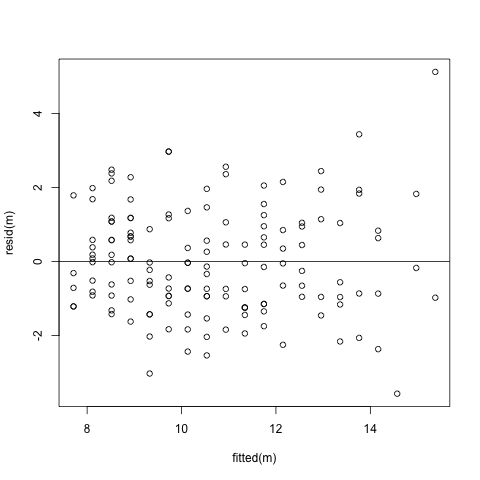
Linearity: Residuals should be centered at 0.
Equal Variance: Variances are similar across fitted values.

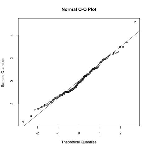
Draw Normal QQ Plot howto plot

QQ stands for Quantile-Quantile.
X axis for theoretical quantiles, Y axis for sample quantiles.

As for checking normality of errors:

X axis goes to the normal distribution quantiles
Y axis goes to the residuals of the model.

m = lm(Hwt ~ Bwt, data = MASS::cats)
qqnorm(resid(m))
qqline(resid(m))

Explanatory function

qqplot = function(e) {
  n = length(e)
  # For n = 10, this vector contains quantiles of [0.05 0.15 0.25 ... 0.95]
  normal_quantiles = qnorm(((1:n - 0.5) / n))
  # plot theoretical verus observed quantiles
  plot(normal_quantiles, sort(e))

  # calculate line through the 1st and 3rd quartiles
  slope     = (quantile(e, 0.75) - quantile(e, 0.25)) / (qnorm(0.75) - qnorm(0.25))
  intercept = quantile(e, 0.25) - slope * qnorm(0.25)
  # add to existing plot
  abline(intercept, slope, lty = 2, lwd = 2, col = "dodgerblue")
}

http://daviddalpiaz.github.io/appliedstats/model-diagnostics.html#q-q-plots

`lmtest::bptest(model, ...)` reference

Perform BP test howto

Test homoscedasticity. (whether or not the error is equally distributed)

m = lm(Hwt ~ Bwt, data = MASS::cats)
lmtest::bptest(m)


  studentized Breusch-Pagan test

data:  m
BP = 9.5294, df = 1, p-value = 0.002022

https://www.rdocumentation.org/packages/lmtest/versions/0.9-36/topics/bptest

`shapiro.test(x)` reference

Perform Shapiro-Wilk Test howto

Unlike other test functions, shapiro.test accepts a vector instead of a lm object.

shapiro.test(rnorm(25))


  Shapiro-Wilk normality test

data:  rnorm(25)
W = 0.91987, p-value = 0.0509

`hatvalues(model, ...)` reference

Calculate Leverage howto

m = lm(mpg ~ hp, data = mtcars)
unname(hatvalues(m))

 [1] 0.04048627 0.04048627 0.05102911 0.04048627 0.03675069 0.04317538
 [7] 0.09757509 0.08046517 0.04958291 0.03510034 0.03510034 0.03886509
[13] 0.03886509 0.03886509 0.05458370 0.06327290 0.07888001 0.07592585
[19] 0.09277415 0.07704010 0.04819161 0.03132530 0.03132530 0.09757509
[25] 0.03675069 0.07592585 0.05253020 0.03903750 0.12568847 0.03675069
[31] 0.27459288 0.04099664

`rstandard(model, ...)` reference

Calculate Standardized Residual howto

Calculates: \[ r_i = \frac{e_i}{s_e\sqrt{1 - h_i}} \]

m = lm(mpg ~ hp, data = mtcars)
unname(rstandard(m))

 [1] -0.42118619 -0.42118619 -0.25341558 -0.31547671  0.14271781 -1.27952886
 [7]  0.24990523 -0.39648860 -0.21698865 -0.66062513 -1.02957426 -0.37436332
[13] -0.13671767 -0.69122419 -1.52076121 -1.34530901  0.07920301  1.83232949
[19]  1.04609436  2.21923491 -0.52556608 -1.14798677 -1.22689309 -0.02259947
[25]  0.27459819  0.45893182  0.56112724  2.11548290  1.02806065  0.40647857
[31]  2.35785298 -0.33359639

`cooks.distance(model, ...)` reference

Find influential observations

Calculates and test the value heuristically:

\[\begin{aligned} D_i &= \frac{1}{p}r_i^2\frac{h_i}{1 - h_i}\\ D_i &> \frac{4}{n} \quad \text{(when it's true, the observation is influential)} \end{aligned} \]

m = lm(mpg ~ hp, data = mtcars)
unname(cooks.distance(m) > 4 / nrow(mtcars))

 [1] FALSE FALSE FALSE FALSE FALSE FALSE FALSE FALSE FALSE FALSE FALSE FALSE
[13] FALSE FALSE FALSE FALSE FALSE  TRUE FALSE  TRUE FALSE FALSE FALSE FALSE
[25] FALSE FALSE FALSE FALSE FALSE FALSE  TRUE FALSE

Calculate Variance Inflation Factors howto

You can use car::vif(model). It appears that many packages include this kind of functions.

m = lm(mpg ~ disp + hp, data = mtcars)
car::vif(m)

    disp       hp 
2.670938 2.670938

Also, we can calculate it manually:

m = lm(mpg ~ disp + hp, data = mtcars)
md = lm(disp ~ hp, data = mtcars)
mh = lm(hp ~ disp, data = mtcars)
c(1 / (1 - summary(md)$r.squared), 1 / (1 - summary(mh)$r.squared))

[1] 2.670938 2.670938

If the VIF of a parameter is larger than 5, heuristically it can be considered to be somewhat collinear to other variables.

Calculate Partial Correlation Coefficient howto

my = lm(mpg ~ disp, data = mtcars)
mh = lm(hp ~ disp, data = mtcars)
cor(resid(mh), resid(my))

[1] -0.3258012

When this value is large, we can think that the unexplained portion of the candidate predictor, hp in the example above, and that of the response are highly correlated. This means that there is no significant collinearity between the candidate predictor and the existing predictors, disp in this case. So, adding the candidate predictor is of benefit.

We can also visualize this relationship:

plot(resid(my) ~ resid(mh))
abline(h = 0, lty = 2)
abline(v = 0, lty = 2)
abline(lm(resid(my) ~ resid(mh)))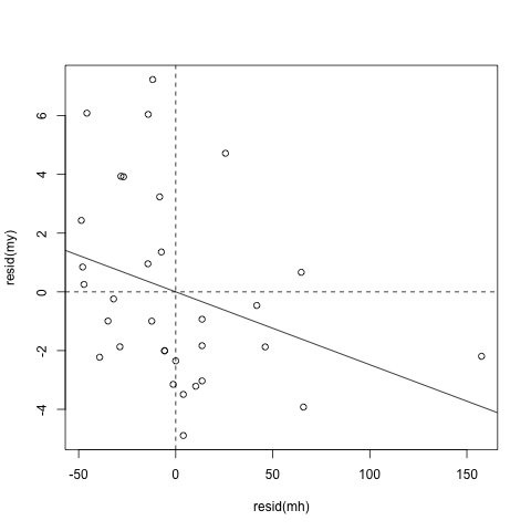

Perform a model selection with exhaustive search howto

Use leaps::regsubsets(formula, data = data)
This returns a list of best models of each size.

`step(object, scope, direction)` reference

Perform a model selection with stepwise search based on AIC/BIC howto

# Backward AIC
selected_model = step(full_model, direction = "backward")
# Backward BIC
selected_model = step(full_model, direction = "backward", k = log(n))
# Forward AIC
selected_model = step(start_model, scope = formula, direction = "forward")
# Both AIC
selected_model = step(start_model, scope = formula, direction = "both")

Note that it is not available to use . in scope. To use . for the scope, you can pass a list to scope as follows:

selected_model = step(start_model, scope = list(upper = end_model), direction = "both")

# Suppress trace
selected_model = step(full_model, direction = "backward", trace = 0)

step function respects the model hierarchy. For example, when we have two-interaction, both first order term should be in the model. Or, when we have a quadratic term, the first order term should be in the model.

Note that step() implicitly refers the dataset which the start_model bases on. So, if you use step() in a function, you should do it as follows:

step_backward = function(start_model) {
  # NOTE: `step()` function implicitly refers the model's data by the name.
  # Generally the data is accessible from the calling frame.
  # So deines a new environment from it.
  e = new.env(parent = parent.frame())
  # Pass the arguments to the new `e`
  e$start_model = start_model
  with(e, {
    n = nobs(start_model)
    list(
      aic = step(start_model, direction = "backward", trace = 0),
      bic = step(start_model, direction = "backward", trace = 0, k=log(n))
    )
  })
}

Calculate AIC, BIC howto

library(faraway)
model = lm(hipcenter ~ Age + Ht + Leg, data = seatpos)

Calculate AIC

extractAIC(model)

[1]   4.0000 274.2418

Calculate BIC

n = nrow(seatpos)
extractAIC(model, k = log(n))

[1]   4.0000 280.7922

It returns c(<equivalent degrees of freedom>, <AIC>).

Perform Leave-One-Out Cross Validation howto

calc_loocv_rmse = function(model) {
  sqrt(mean((resid(model) / (1 - hatvalues(model))) ^ 2))
}

Extract the number of observations from a fit howto

nobs(fit)  # Which is equal to `nrow(data)`

https://stat.ethz.ch/R-manual/R-devel/library/stats/html/nobs.html

Change the null hypothesis to \(H_0 = T\) in `summary(lm)` howto

By default, summary() calculates p-value of \(H_0: \beta = 0\). So we need to modify the formula for the model as follows:

summary(lm(y ~ x, offset = T*x))  # testing against slope=T
summary(lm(I(y - T*x) ~ x))       # testing against slope=T

Table of Contents